Volatility based initial MMS for Sugar
Figure 4.15 Largest losing trade for sugar using the 65sma-3cc trading system increases as the volatility-based initial money management stop increases.
also the short exit, and vice versa. At this stage, the goal of the filter is only to reduce some of the signals in a congestion area.
You can design many types of filters. Here we use a momentum-based filter using the range action verification index discussed earlier. The RAVI is the absolute percentage difference between the 7-day and 65-day simple moving averages of the daily close. This n-eans that when the market is in a congestion or consolidation phase, th • short (7-day) and long (65-day) moving averages tend to be close together. Conversely, when the markets are trending, these averages are far apart.
You can also use Wilder's ADX (average directional index) as a filter for trending or nontrending markets. Specifically, if the ADX is declining, and/or below 20, then you can assume that the market is consolidating or entering a congestion phase. You could also use the .r-day high-low range, or other momentum oscillators, to diagnose market conditions. Remember that any indicator you use, including the RAv^I, will not work perfectly every time.
First, let us briefly review the performance of 65sma-3cc trading system in consolidating markets. As prices begin to trade in a narrow
The 65sma-3cc Trend-Following System 95
| 106*08 |
| •IOI*W |
| •lOO'OO |
| •WM |

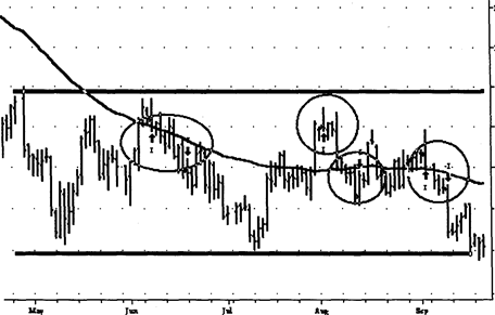
Figure 4.16 The 65sma-3cc trading system generated several entry signals as the U.S. bond market consolidated after its now-famous bear market tumble. The circled areas show the six signals—three long entries and three short entries—in this broad consolidation region.
range, without a definite direction, the longer moving average (65sma) flattens out. Prices oscillate on either side of this average. Hence, you can get a succession of long and short signals as the market posts three consecutive closes above or below the 65sma.
In some sense, this becomes a self-correcting process, because the entry signals are not very far apart in price. Hence, even though you will have several losing trades in succession, the amount of the losses will be relatively small. You can imagine that in some cases the market will trade within a broad trading range, with sharp, but quick moves in '30th directions. The U.S. bond market has a tendency to form such consolidations. This is a worst-case scenario for the 65sma-3cc system because you will get short-lived entry signals but incur relatively large losses, since the market is making choppy moves that quickly span the trading range. Some examples of such market action follow.
Figure 4.16 shows the September 1994 U.S. bond contract consolidating after its now-famous bear market. Observe the six "false" signals from the system. Since the market was in a broad trading range, and prices were moving about on either side of the average, the false signals are inevitable given our definition of the trading system. This is a good illustration of a general principle: Whatever conditions you define, markets can always find ways to trigger false signals.
96 Developing New Trading Systems
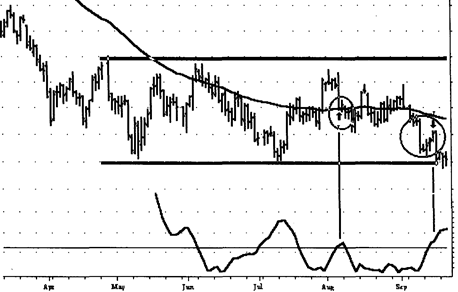
Figure 4.17 shows the results of the same trading system with a filter. Now there are only two trades in the congestion region. The RAVI is plotted under the prices, so you can see that the signals occurred in regions where the RAVI was greater than 1. Since the model was already short coming into the picture, the first trade is a buy. The filtered model could generate a buy signal only if RAVI was greater than one and there were three consecutive closes above the 65sma.
A tight consolidation region developed immediately after the buy signal, dropping the RAVI below 1. Hence, this filtered out the next two signals, a sell and then a buy. Similarly, it also filtered out a buy signal and a sell signal in June. The last sell signal occurred when the RAVI climbed above 1 and there were three consecutive closes below the 65sma. Thus, we used the level of the RAVI to filter out some whipsaw signals.
What should be the barrier value for the RAVI to filter out signals? There is no perfect answer to this question; you will have to pick a value using one method or another. Raising the RAVI barrier to 1.5 from 1 will filter out even more trades. As Figure 4.18 shows, this model would have been short from the previous October 1993, all the way down and through two major consolidation areas, for a per contract profit of $13,696. Notice how the RAVI rose strongly above 1 when the trend
| .109*12 -I07*M -lOttS -lMf'11 -103*04 -101*15 -100*00 -98*H -2.0 -1.60 -0.80 |

Figure 4.17 Adding a RAVI filter with barrier equal to 1.0 eliminates four of the six false trades in this broad congestion region. Notice that the 65sma-3cc model is fired only if RAVI is greater than 1 in both remaining instances.
The 65sma-3cc Trend-Following System 97

Figure 4.18 Increasing the RAVI filter barrier to 1.5 eliminates even more trades.
gathered strength, peaking just before the start of the lower consolidation phase.
These figures illustrate that you can use a filter to reduce the number of trades from a trend-following model. You can use different filters, and for a given filter you can use different barrier levels. Note that this system still is in the market at all times: either long or short.
By now, the effects of adding a filter should be clear: (1) We filter out some false signals; (2) we can reduce the maximum intraday drawdowns; (3) we can improve the profit factor of a system, i.e., the ratio of gross profit to gross loss over the test period; (4) the average trade usually increases; and (5) the length of the average winning trade increases. Our results will depend on how we choose the filter and its barrier level.
These comments can be supported with more data. Table 4.4 shows the results of calculations for adding a 0.5 percent RAVI filter to the 65sma-3cc model with a $1,000 initial stop and $100 deducted for slippage and commissions for 14 arbitrarily selected markets. These markets are a broad basket of softs, grains, metals, energies, currencies, and index and interest rate contracts. You can compare them to Table 4.2 for an estimate of their performance without stops or filters.
Table 4.5 shows the effect of the 0.5 percent RAVI filter on the dollar value of the average trade. The filtered system has a higher average trade, reflecting the improved quality of the entries.
98 Developing New Trading Systems
Table 4.4 Effect of adding a filter of RAVI = 0.5 to the 65sma-3cc system;
filtering reduces the number of trades
| Number | ||||||
| Number | Number | of | ||||
| Paper | Number | of | of Trades | Winners | ||
| Profit | of Trades | Winners | (No | (No | ||
| Market | Test Period | ($) | (Filtered) | (Filtered) | Filter) | Filter) |
| British pound | 2/75-7/95 | 111,106 | ||||
| Corn | 2/75-7/95 | 26,613 | ||||
| Crude oil | 3/83-7/95 | 2,150 | ||||
| Deutsche mark | 2/75-7/95 | 49,613 | ||||
| Eurodollar | 2/82-7/95 | 11,775 | ||||
| Gold | 2/75-7/95 | 36,690 | ||||
| Silver | 2/75-7/95 | 152,585 | ||||
| S&P-500 | 4/82-7/95 | 59,310 | ||||
| Sugar | 2/75-7/95 | 29,055 | ||||
| U.S. bond | 8/77-7/95 | 31,588 | ||||
| 10-year T-note | 5/82-7/95 | 16,750 | ||||
| Wheat | 2/75-7/95 | -2,040 |
Tables 4.4 and 4.5 show that as you filter a trading system, the number of trades decreases, the average trade increases, and the profit factor improves. These results are sensitive to the filtering rules. You can choose to filter a system many different ways. For example, you can use
Table 4.5 Adding a filter increases the average trade
| Average Trade | Average Trade | |
| Market | (No Filter) (S) | (Filtered) (S) |
| British pound | 1,269 | 1,543 |
| Corn | ||
| Coffee | 2,783 | 3,488 |
| Crude oil | -66 | |
| Deutsche mark | ||
| Eurodollar | ||
| Gold, Comex | ||
| Silver | 1,014 | 1,426 |
| S&P-500 | ||
| Sugar | ||
| U.S. bond |
The 65sma-3cc Trend-Following System 99
the ADX instead of the RAVI. Again, you have to make trade-offs in every choice you make.
In summary, we took the 65sma-3cc trend following system and tested its performance over 20 years of data and 23 markets. Then, we analyzed the winning and losing trades to select an initial money management stop. We filtered the system to reduce the number of signals. We used a "one-way" model, which does not allow back-to-back long or short trades. The main advantage of using a one-way model for testing is that it allows an apples-to-apples comparison of changes in trading strategy. You do not need this restriction for actual trading.
We have not tried to manage the equity curve in each of our analyses; the system was allowed to run to maximize profits. However, this system was always in the market. If we add a neutral zone, the system will not be always in the market. We can also consider adding one or more exit rules to get a smoother equity curve. With a bit of luck, the exit strategy will also create a neutral zone.